Crowd detection using fractal dimension and local density

In this post, I will present my university project on crowd detection. This project has been realized during my second master’s degree at Paris-Descartes University (Vision and Intelligent Machine specialization).

Crowd detection is the task of classifying and localizing a crowd in images (see Fig. 1). In this project, I am particularly interested in pedestrians crowd detection. I mostly used image processing methods to isolate the crowd from non-interesting objetcs and background. Specifically, the classification task is based on fractal dimension and the localization task is based on local density.

Figure 1: Example of crowd detection using my solution.

1. Applications of crowd detection

According to Google Scholar, 1460 papers have been published concerning crowd detection at this day. There are a myriad of areas where crowd detection is useful [5]. The figure Fig. 2 shows some of these areas.

Thanks to the amazing progress of technology in the medical field, cancer patients can more and more be saved. Detecting a certain number of cancerous cells, thus forming a crowd, may help for an early-stage diagnosis.

Disaster management generally concerns overcrowding scenarios such as music events. If any panic breaks out among a crowd of thousands of persons, their lives are definitely in danger. Detect overcrowded areas as earlier as possible may avoid the worst scenario.

In addition, crowd detection enables safety and monitoring procedures to be automated. It can be very helpful to detect anomalies and thereby predict risks.

Moreover, crowd detection is valuable for public event management. The supervisory authorities will receive a notification as soon as a public demonstration occures. Therfore, this will greatly assist them to restore calm and order.

Another significant case where crowd detection can be relevant comes to track suspicious activity. For instance, people who are fighting necessarily attract other people and this may exacerbate the situation. So, with crowd detection the security officials receive information regarding suspicious activity in the area, and thus can rapidly intervene.

Figure 2: Applications of crowd detection in different areas.

2. Model architecture

In this section, I will explain, step by step, how to build a crowd detection pipeline entirely based on image processing methods. The pipeline consists of 2 components. The first component concerns crowd classification and the second one concerns crowd localization. I will develop in the following sub-sections each component in detail.

2.1 Crowd classification

In this project, the crowd classification problem is resolved using fractal dimension. But, before proceeding with classification problem, I would like to present the fractal dimension concept.

2.1.1 Fractal dimension

A. Backes et al. explains the concept of fractal dimension as: “A measure of how fast the length of a curve increases as the size of the measuring stick is shortened” [2]. And Robert L. Devaney defines the fractal dimension as: “A measure of how complicated a self-similar figure is” [3].

There are several ways to compute the fractal dimension. I have chosen the box counting method, aka Minkowski-Bouligand Dimension. The fractal dimension (FD) is given by:

$$ FD = \lim_{r\to 0} \frac{log(N(r))}{log(\frac{1}{r})}$$

Where \(N\) is the number of required boxes to cover the fractal and \(r\) is the boxes side.

The choice of the boxes side parameter is crucial. In fact, when \(r\) is too small, the fractal dimension becomes very accurate. However, if \(r\) becomes too big, the fractal may not be correctly covered by the boxes and this surely yields to imprecise results.

In practise, fractal dimension is widely employed to measure and estimate costline mapping. If the goal is to compare which among Australia and Great Britain has the biggest coastline, it would be enough to compute the FD of each map and the one having the biggest FD will be considered as the map with the biggest coastline.

2.1.2 Fractal dimension-based model for classification

Drawing on the previous coastline estimation example, now let’s see how fractal dimension can help with crowd classification.

Crowd classification consists of analyzing an image and saying whether it contains a crowd or not. In this project, a crowd is considered as a grouping of at least 5 persons. If a crowd is correctly extracted from an image with its irregular contours, the fractal dimension of these contours can be computed.

Imagine a scene with only 4 persons. Relying on box counting method, the 4 persons should be coverd by a sufficient number of boxes in order to get a precise fractal dimension. If more than 4 persons are present in the scene, the computed fractal dimension naturally increases. Assuming this, the crowd classification problem is represented by a thresold filtering on the computed fractal dimension. Let \(t_{FD}\) be the threshold on the crowd fractal dimension, the classification is built as follows :

\[y = \left\{ \begin{array}{ll} crowd & \mbox{if } FD >= t_{FD} \\ no \: crowd & \mbox{otherwise} \end{array} \right.\]

2.1.3 Crowd classification pipeline

The crowd classification process can be divided into 4 steps (see figure Fig. 3).

First of all, the color image \(I\) is read. Then, \(I\) goes through a chain of preprocessing functions. The edges are extracted from \(I\) using OpenCV’s preprocessing function called \(cv2.dnn.blobFromImage\). This function performs, among others, Mean Subtraction which serves to normalize the image and helps reducing illumination changes. Then, binarization is performed using \(cv2.adaptiveThreshold\).

The next step is contours detection which is the most important preprocessing function. Because this step draws the borders on which \(FD\) is directly computed. The contours are detected using \(cv2.findContours\). Sometimes, the obtained contour map seem to have contours on the borders of the image which is unnecessary. A manual operation is added in order to delete these specific contours. Finally, the classification decision is formulated according to the comparison between FD and \(t_{FD}\).

Figure 3: Crowd classification pipeline.

2.2 Crowd localization

The crowd localization in this project is defined according to the local density. Naturally, crowded scene contains a high density compared with a scene containing a few people. The local density is computed from the contour map. Then, it is thresholded and used to create the bounding box. The bounding box is a set of rectangles which covers the crowd if it exists.

Now, let’s dive into an elaborated description of the crowd localization pipeline. This pipeline consists of a chain of 5 steps (see figure Fig. 4).

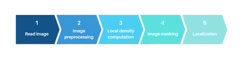
Figure 4: Crowd localization pipeline.

First, the color image \(I\) is read. Contrary to the classification process, \(I\) is smoothed before the edges are extracted. Smoothing helps to reduce noise and details that are meaningless for the localization problem such as facial features. After that, the edges are extracted and binarizzd in the same way as for classification. Next, the contours are detected following the same method as for classification.

The next step is the local density computation. As \(I\) has already been binarized, it only contains white pixels (constituting the contours) and black pixels (constituting the background). So, the contour map is devided into patches and on each patch the number of white pixels is accounted and saved into a matrix. Let \(M\) be the resulting matrix which has the same size as the number of patches. \(M\) represents the local density matrix.

Let \(t_{LD}\) be a threshold on the local density. \(t_{LD}\) is used to filter \(M\) and to keep the most dense patches. The kept patches reflect the pentential regions where a crowd may be located. After that, the kept patches are binarized and resized to the dimension of the original image in order to form the mask. Finally, the mask is used to draw the bounding box around the crowd.

2.3 Visual illustration of crowd detection pipeline

In the two previous parts, I have explained how the classification and the localization are performed. In this part, I suggest to illustrate with the figure Fig. 5 the complete crowd detection pipeline.

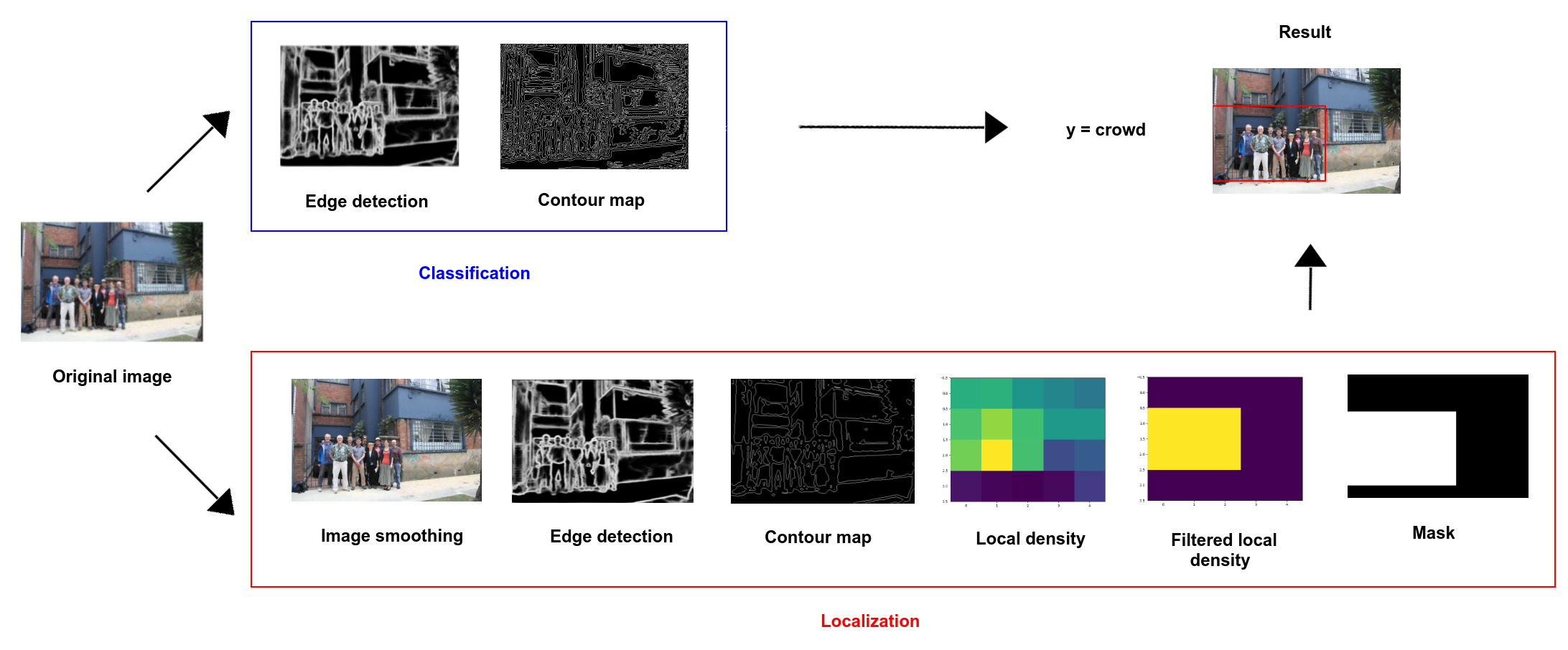
Figure 5: Illustration of the complete crowd detection pipeline.

As shown in the figure Fig. 5, the edge detection step is shared between the 2 separate branches of classification and localization. For the classification and localization, only relevant steps are represented such as masking image or contour map. At the end, the result is given by the class (crowd or no crowd) and the bounding box in red.

2.3 Model implementation and software requirements

• The entire code is written in Python 3.8.5.
• OpenCV 4.4.0 is the main used library for image processing.
• GPU is not required.

2.4 Dataset

CrowdHuman is a benchmark for detection human in a crowd [4]. It has been created by Shuai Shao et al. in 2018. This benchmark includes some images which are not free. These particular images are protected with a special writing on it. This may distort the contour map and produce misleading results. To solve this problem, I have simply deleted the protected images.

After cleaning the benchmark, only few images were kept. So, I was obliged to search for another dataset.

The second benchmark I have studied is CityStreet [6][7]. CityStreet has been published in 2019 by Qi Zhang et al. Unlike CrowdHuman, CityStreet contains images of people which are sometimes so far from the camera. As I did not managed multi-scale images, I was brought to work only with images of the same scale. So, I only kept few images where people are close to the camera.

Then, I have noticed that the majority of the kept images represented crowded scene. To leveling this problem, I have picked some images from Mask Dataset [1].

A total of 715 images are selected for the optimization phase. 505 images are dedicated to the class “crowd” and 210 images are dedicated to the class “no crowd”.

For the test phase, 447 images are selected. 360 images are dedicated to the class “crowd” and 87 images are dedicated to the class “no crowd”.

The figure Fig. 6 shows some examples of the resulted dataset.

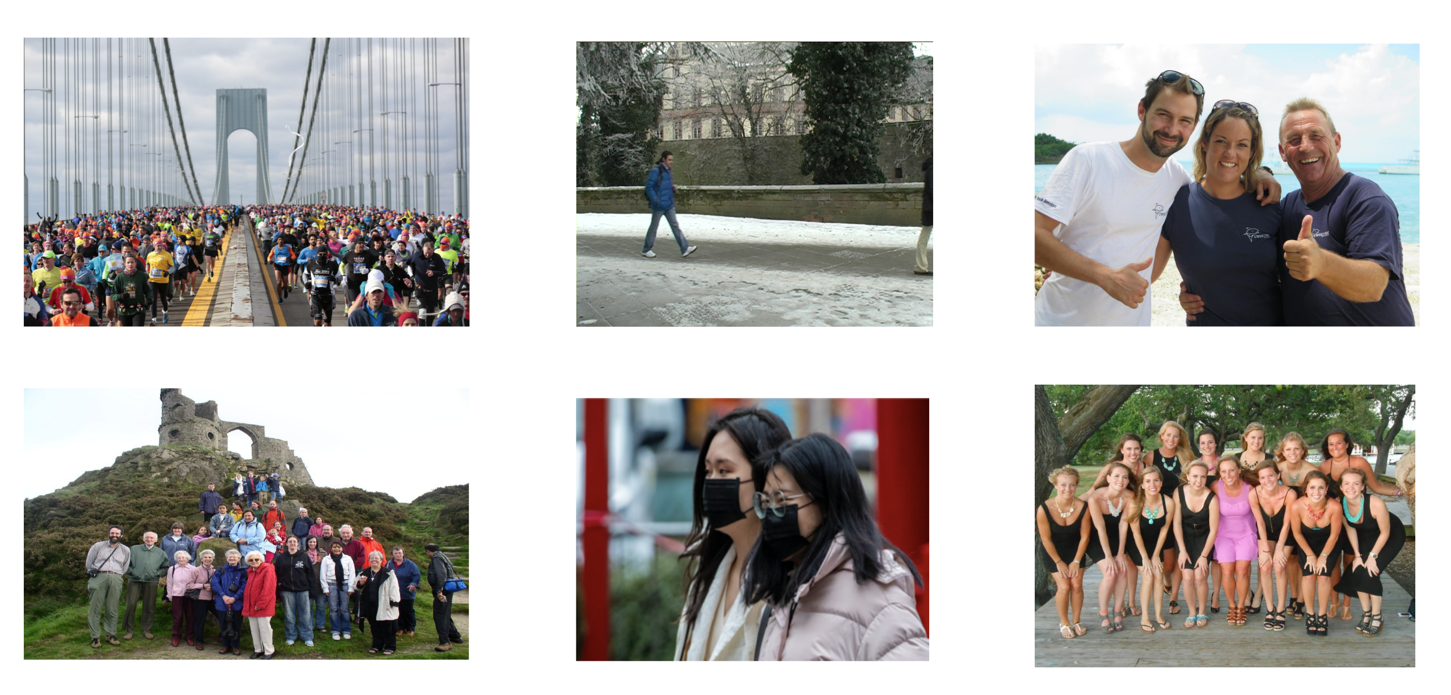
Figure 6: Some examples of the constructed dataset.

2.5 Parameters optimization

The optimization step consists of determining the two parameters \(t_{FD}\) (fractal dimension threshold) and \(t_{LD}\) (local density threshold). Let’s begin with \(t_{FD}\).

2.5.1 Fractal dimension threshold optimization

For each image from the dataset, the first three steps are performed (read image, image preprocessing and fractal dimension computation). The figure Fig. 7 shows the fractal dimension values of the entire dataset. For example, approximately 6 images have a fractal dimension of 1.7.

Figure 7: Plot of fractal dimension values of the entire dataset.

\(t_{FD}\) should be thoroughly chosen. It should be picked from the interval delimited by the red rectangle (see figure Fig. 7). This interval represents the boundaries between “crowd” and “no crowd” classes.

Now let’s take a closer look at this interval. 8 classification experiments have been realized using each threshold of the interval [1.70;1.77]. The figure Fig. 8 shows the True Positive (TP) and the False Negative (FN) for each class and for each threshold.

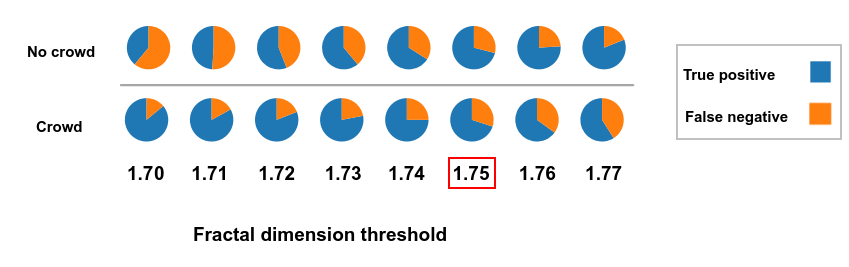
Figure 8: Test of different fractal dimension thresholds and their impact on the classification performance.

If \(t_{FD} = 1.70\), the images containing a “crowd” are correctly classified with a percentage of 87%. However, 67% of images with “no crowd” are classified as “crowd”. So this thresold does not allow balancing between classification performance for each class. The best value that permits such balance is when \(1.75\). In this case, the TP of “crowd” images consist of 72% and the TP of “no crowd” images consist of 70% (betwen TP and FN).

Thus, the value of the fractal dimension threshold is set to \(t_{FD} = 1.75\).

Now, let’s move on to local density threshold optimization.

2.5.2 Local density threshold optimization

The optimization of the local density threshold is different from the optimization of the fractal dimension threshold. \(t_{LD}\) filters the number of white pixels within a given patch of the image. It takes a value in the interval [0,1]. Concretely, the number of white pixels is computed for each patch. Let \(max_{patch}\) be the maximum number of white pixels. If the number of white pixels of a given patch is greather than \(max_{patch}\) x \(t_{LD}\), then the patch is kept to be used later to construct the mask.

To optimize \(t_{LD}\), I have performed the localization process many times. Each time, \(t_{LD}\) was set to a different value. At the end of the process, the \(t_{LD}\) which allows the best localization is selected. Thus, the value of the local density threshold is set to \(t_{LD} = 0.7\).

2.6 Evaluation

In this part, I will define some metrics to evaluate the proposed solution. After that, I will present quantitative and qualitative results.

2.6.1 Evaluation metrics

To evaluate the crowd classification solution, I have used Mean Squared Error (MSE) which is given by:

$$ MSE = \frac{1}{n}\sum_{i=1}^{n}(y_{i_{real}} - y_{i_{predicted}})^2 $$

Where \(n\) is the dataset size, \(y_{i_{real}}\) is the real class of the image \(i\) and \(y_{i_{predicted}}\) is the predicted class of the image \(i\).

Just for simplification, I have defined a personal metric (inspired from IOU) to evaluate the crowd localization process. The metric is given by:

$$ Loc_{metric} = \frac{size(P_{real} ∩ P_{predicted} )}{size(P_{real} ∪ P_{predicted} )} $$

Where \(P_{real}\) are the real patches and \(P_{predicted}\) are the predicted patches.

If \(P_{real} ∩ P_{predicted} = P_{real}\) then \(Loc_{metric} = 1\).

If \(P_{real} ∩ P_{predicted} = Ø\) then \(Loc_{metric} = 0\).

So, \(Loc_{metric} ∈ [0,1]\)

2.6.1 Quantitative results

Here are some statistics on both optimization and test phases. The table below shows the obtained results (figure Fig. 9).

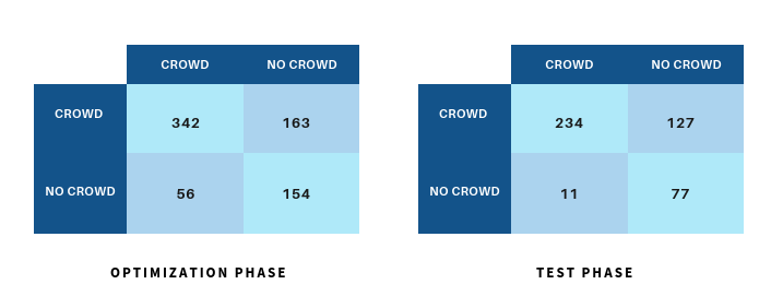
Figure 9: Statistics on optimization and test phases.

For the optimization phase, the method classifies correctly 342 crowded images among 361 crowded images. 154 uncrowded are correctly classified among 210 images. In addition, I have found \(MSE = 0.306\) and \(Loc_{metric} =0.66\).

For the test phase, the method does better for the uncrowded images but for the crowded images, the results od the optimization phase are better. The computed \(MSE\) is approximately identic to the \(MSE\) obtained at the optimization phase. So, \(MSE = 0.307\). And I have found \(Loc_{metric} =0.68\) which is also very close to the obtained result at the optimization phase.

Then for the metrics,

I have calculated \(MSE\) and \(Loc_{metric}\) on the training and test datasets.

2.6.1 Qualitative results

Now, let’s analyze some qualitative results.

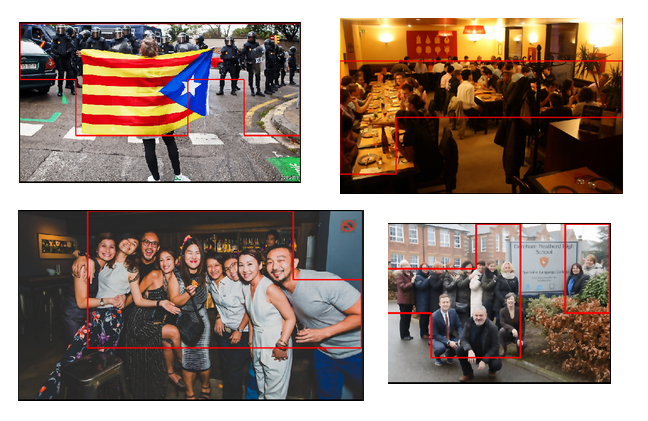
Figure 10: Qualitative results (part 1).

The figure Fig. 10 shows some results of the crowd detection process. The first thing to notice is that the proposed solution allow the bounding box to take an irregular form. Which means that it is not obliged that the bounding box be of a rectangular form.

In addition, almost all classical deep learning methods use rectangular bounding box. Such a mothd would cover the crowded area in the image on the top right of the figure Fig. 10 with a bigger rectangular bounding box as shown in the figure Fig. 11. The result is less precise than mine.

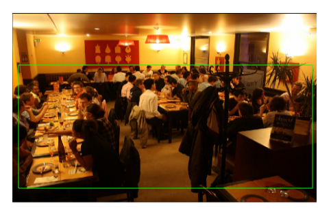
Figure 11: A potential prediction by a deep learning based model.

But this method presents some weaknesses. First, if there are some trees or buildings the result is less accurate (see figure Fig. 12). These areas are strongly textured and by the way present a high contours regions.

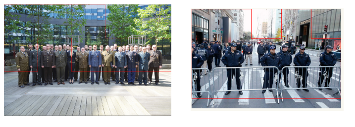
Figure 12: Qualitative results(part 2).

Also, is an image is taken with a focus in the center of the image for example, the other regions are naturally blurred. The figure Fig. 13 shows this case. Consequently, the blurred areags will not be detected.

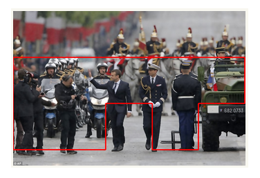
Figure 13: Qualitative results(part 3).

2.7 Running the Application

I have deployed the solution via Heroku as a web application. To test the application, click on this link Crowd Detection App.

The figure Fig. 14 illustrates the web application page.

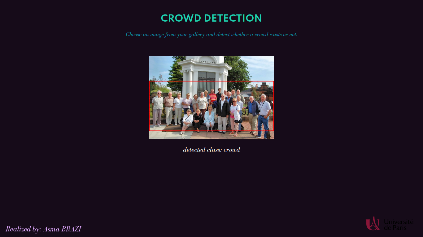
Figure 14: Crowd detection web application.

Conclusion

The proposed solution is still far from saturating the benchmark metrics. If complicated backgrounds are crossed, the model may miss targets or may provide an imprecise bounding box. However, the model is only based on image processing methods for the task of crowd detection. In fact, no intelligence is behind the established process.

As future works, here are some potential areas to be explore :

• Dataset augmentation.
• Multiscale effects management.
• Improve the localization precision.

You can access the complete code via the GitHub repository.

References

[1] Mask dataset. https ://makeml.app/datasets/mask, 2020

[2] A. Backes and O. Bruno. Fractal and multi-scale fractal dimension analysis : a comparative study of bouligand-minkowski method.ArXiv, abs/1201.3153, 2012.

[3] Robert L. Devaney. Fractal dimension. http ://math.bu.edu/DYSYS/chaos-game/node6.html,1995.

[4] Shuai Shao, Zijian Zhao, Boxun Li, Tete Xiao, Gang Yu, Xiangyu Zhang, and Jian Sun. Crowd-human : A benchmark for detecting human in a crowd.arXiv preprint arXiv :1805.00123, 2018

[5] Nilam Sjarif, Siti Mariyam Shamsuddin, Siti Mohd Hashim, and Siti Yuhaniz. Crowd analysis and its applications. volume 179, pages 687–697, 01 2011.

[6] Qi Zhang and Antoni B Chan. Wide-area crowd counting via ground-plane density mapsand multi-view fusion cnns. InProceedings of the IEEE Conference on Computer Vision andPattern Recognition, page 8297–8306, 2019.

[7] Qi Zhang and Antoni B Chan. Wide-area crowd counting : Multi-view fusion networks forcounting in large scenes. Inhttps ://arxiv.org/abs/2012.00946, 2020